Summary
Given a corpus of documents, the premise in Natural Language Processing Topic Extraction is that each word in each document has a latent assignment into one of \(K\) possible topics. A standard in the literature to estimate these topics is to use Latent Dirichlet Allocation (LDA) (Blei et al (2003)). In a nutshell, LDA clusters words into topics, which are distributions over words, while at the same time classifying articles as mixtures of topics.
The Model
LDA’s generative model assumes a latent structure consisting of a set of topics upon which each document is produced by choosing a topic according to the distribution of topics in the corpus, and then each word in this document is generated using a distribution over words associated with this particular topic.
The first step is to represent a corpus of documents by mathematical objects so we can model the probabilistic structure of topics and words. Consider a corpus of \(D\) documents made of words from a dictionary containing \(V\) terms (Usually \(V\) will be used to the denote the dictionary, that is the set of terms and its dimension); we represent a document \(d\) with \(w_{d}\), a vector \(w_d\in\mathbb{N}^{n_d}\), where \(n_d\) is the number of terms in document \(d\) such that each entry in this vector \(w_d=(w_{d1},...,w_{dn_d})\), \(w_{di}\) stands for the index within the dictionary \(V\) of the word in position \(i\) of the document.
In (Blei et al (2003))’s LDA model the premise is that there is a latent assignment of documents into topics with a mixed membership based on two principles:
- that every document is a mixture of topics and
- that every topic is a mixture of words.
To clarify the previous principles we need to introduce more notation. Let \(K\) be the number of latent topics in the corpus; this is a number picked by the researcher that is guided by metrics discussed later. Moreover, let \(\theta_d\) a vector in the \(K\) dimensional simplex \(\Delta^{K-1}\) so \(\theta_{dk}\in[0,1]\) stands for the share of topic \(k\) in document \(d\), reflecting that there is a mixed membership into topics. On the other hand, let \(\beta_k \in \Delta^{V-1}\) be the vector of term-probabilities in topic \(k\); that is \(\beta_{kv}\in[0,1]\) is the probability of observing word \(v\) in a generic document with full membership into topic \(k\). This means that we consider two topics as distinct from each other if they differ on the frequency (probability) with which at least one term appears in each topic; that is topics are mixtures of words.
To connect the previous two probabilistic statements, we consider a latent variable \(z_{d,n}\) associated with word \(n\) in document \(d\), \(w_{d,n}\), such that \(z_{d,n}\in (1,...,K)\) is the topic assignment of \(w_{d,n}\). With this notation, and considering a Dirichlet prior for \(\beta_k\in \Delta^{V-1}\), \(Dir(\beta|\eta)\) with hyperparameter \(\eta\in \Delta^{V-1}\) and another Dirichlet prior for \(\theta_d\in \Delta^{K-1}\), \(Dir(\theta_d|\alpha)\) with hyperparameter \(\alpha\in \Delta^{K-1}\), the LDA model generates documents for a corpus \(D\) in the following fashion:
- Draw \(K\) vectors \(\beta_k\in\Delta^{V-1}\) from \(Dir(\beta_k|\eta)\).
- Draw \(D\) vectors \(\theta_d\in\Delta^{K-1}\) from \(Dir(\theta_d|\alpha)\).
- Each word \(w_{d,n}\) in document \(d\) is generated in two steps:
- Draw \(z_{n,d}\in (1,...,K)\) according to topic probabilities \(\theta_d\).
- Draw \(w_{d,n}\) using term probabilities \(\beta_{z_{n,d}}\).
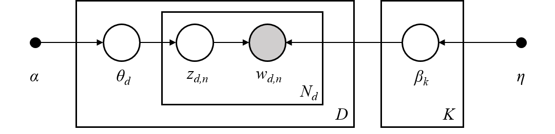
Figure 1: LDA Graphical Model
These dependencies can be summarized in the graphical model depicted in Figure 1. Following the Bayesian network, the posterior likelihood over latent variables given an observed corpus \(\{w_{d,n}\}\) and hyper parameters \(\eta, \alpha\) is given by \[\begin{align} L:=p(z,\theta, \beta|w,\alpha,\eta)&\propto\left[\prod_{d,n} p(w_{d,n}|z_{d,n}, \beta)\right] \left[\prod_{d,n} p(z_{d,n}|\theta_d)\right] \\\\ &\times \left[\prod_{d}p(\theta_d|\alpha)\right]\left[\prod_k p(\beta_k|\eta)\right] \end{align}\]
where \(w=(w_{d,n})\), \(z=(z_{d,n})\), \(\beta\) is a \(V\times K\) matrix of term probabilities with column \(k\) given by \(\beta_k\) and \(\theta\) is a \(K\times D\) matrix of topic memberships with column \(d\) given by \(\theta_d\). The goal of the estimation step is to do inference on the posterior distribution above. Two of the most used methods for doing so rely on a Variational Expectation Maximization Algorithm (see Blei et al (2017) for a review) and Gibbs sampling.
Gibbs Sampling Details
Following the Bayesian network in Figure 1, it can be noted that the Markov blanket for \(\theta_d\) is \((\alpha, z_d)\); the Markov blanket for \(\beta_k\) is \((\eta, w, z, \beta_{-k})\), where \(\beta_{-k}\) is the matrix of term probabilities with \(\beta_k\) is removed and finally the Markov blanket for \(z_{n,d}\) is \((\theta_d, w_{d,n}, \beta)\). Then the Gibbs sampling strategy for \(p(z,\theta, \beta|w,\alpha,\eta)\) follows:
- Initialize \(z^0, \theta^0\) and \(\beta^0\).
- In iteration \(i\):
Sample \(z^i\) from \(p(z|w,\beta^{i-1}, \theta^{i-1})\).
In the case for topic assignment \(k\) and term \(v\) by Bayes theorem: \[\begin{align} P[z_{d,n}=k| w_{d,n}=v,\beta,\theta_d]&\propto P[w_{d,n}=v|z_{d,n}=k,\beta, \theta_d]\\\\ &\times P[z_{d,n}=k|\beta, \theta_d]=\beta_{k,v}\theta_{d,k} \end{align}\]
Meaning that \(P[z_{d,n}=k| w_{d,n}=v,\beta,\theta_d]=\frac{\beta_{k,v}\theta_{d,k}}{\sum_{\tilde{k}} \beta_{\tilde{k},v}\theta_{d,\tilde{k}}}\), so sampling each \(z_{d,n}\) can be seen as a draw from a multinomial distribution conditional on observed \(w_{d,n}=v\), and on \(\beta^{i-1}, \theta^{i-1}\).
Sample \(\theta^i\) from \(p(\theta|\alpha, z^{i-1})\).
Let \(n_{d,k}=\sum_n \mathbb{I}( z_{d,n}=k )\) be the number of words in document \(d\) that have topic allocation \(k\). Then by Bayes theorem \(p(\theta_d|\alpha,z_d)\propto p(z_d|\theta_d)p(\theta_d|\alpha)\) where \(p(\theta_d|\alpha)\) is known (a Dirichlet distribution) and
\[p(z_d|\theta_d)=\prod_n \sum_k \mathbb{I}\{ z_{d,n}=k \} \theta_{d,k}=\prod_k \theta_{d,k}^{n_{d,k}}\] so sampling \(\theta^i\) requires sampling from a Dirichlet distribution \(Dir(\theta|\tilde{\alpha})\) with parameter \(\tilde{\alpha}=(\alpha_1+n_{d,1},..., \alpha_K+n_{d,K})\).
Sample \(\beta^i\) from \(p(\beta|w,\eta, z^i, \beta^{i-1}_{-k})\).
By Bayes theorem \(p(\beta_k|z,w,\eta,\beta_{-k})\propto p(z,w|\beta)p(\beta_k|\eta)\). Let \(m_{k,v}=\sum_{n,d} \mathbb{I}(z_{d,n}=k)\mathbb{I}(w_{d,n}=v)\) be the number of times topic \(k\) allocation variables generate term \(v\), so
\[\begin{align} p(z,w|\beta)&=\prod_{n,d}\sum_{v,\tilde{k}} \mathbb{I}(w_{d,n}=v)\mathbb{I}(z_{n,d}=\tilde{k})\beta_{\tilde{k},v}= \prod_{v,\tilde{k}} \beta_{\tilde{k},v}^{m_{\tilde{k},v}}\\\\ &=\prod_v \beta_{k,v}^{m_{k,v}} \left[ \prod_{v,\tilde{k}\neq k} \beta_{\tilde{k},v}^{m_{\tilde{k},v}} \right] \propto \prod_v \beta_{k,v}^{m_{k,v}} \end{align}\]
which suggests that we sample \(\beta_k\) from a Dirichlet distribution \(Dir(\beta|\eta + m_{k,j})\).
- Repeat step (2) until convergence and burn-in the sample.
There is a computationally cheaper version of the previous Gibbs sampling strategy proposed by Griffiths and Steyvers (2004), a collapse sampling consisting of integrating out \(\theta\) and \(\beta\) from the posterior \(P[z_{d,n}=k| w_{d,n}=v,\beta,\theta_d]\) and just sample \(z\) in each iteration. Letting the \('-'\) superscript denoting counts excluding \((d,n)\) term is possible to show that: \[\begin{equation} \label{eq_collapsedGibbs} P[z_{d,n}=k|z_{-(d,n)},w,\alpha,\eta]\propto \left[\frac{m_{k,w_{d,n}}^-+\eta}{\sum_v m_{k,v}^-+\eta V}\right] \left[\frac{n_{d,k}^-+\alpha}{\sum_{\tilde{k}} n_{d,\tilde{k}}^-+\alpha K}\right] \end{equation}\]
which suggest that once we sample \(z_{d,n}\) then we can construct \(m_{k,v}\), \(n_{k,v}\) and then set: \[\begin{align*} \hat{\beta}_{k,v}&=\frac{m_{k,v}+\eta}{\sum_{\tilde{v}} (m_{k,\tilde{v}}+\eta)}\\\\ \hat{\theta}_{d,k}&=\frac{n_{d,k}+\alpha}{\sum_{\tilde{k}} (n_{d,\tilde{k}}+\alpha)} \end{align*}\]
On selecting the number of topics for LDA
On metrics guiding the selection of \(K\), the number of underlying topics in the corpus, we briefly summarize the following methods proposed:
Griffiths and Steyvers (2004):
The authors propose a Bayesian model selection approach where \(K\) is selected to maximize \(p(\{w_{n,d}\}|K)\). The strategy they propose is to sample topic assignments \(z_{n,d}\) from the collapse Gibbs sampling equation (For doing this it is necessary to run different chains and sample only after burning-in the chain, to allow the chain is mixed enough to the target distribution), and then use such draws to evaluate \(p(w_{n,d}|z_{n,d},T)\). It turns out there is a closed form for the previous posterior given by the fact that \(p(w|z,\beta)\) and \(p(\beta|\eta)\) are conjugate distributions:
\[p(\{w_{n,d}\}|z_{n,d},K)=\left[\frac{\Gamma(V\eta)}{\Gamma(\eta)^V}\right]\prod_{k=1}^K \left[\frac{\prod_{v\in \{w_{n,d}\}}\Gamma(m_{k,v}+\eta)}{\Gamma(\sum_{\tilde{v}} (m_{k,\tilde{v}}+\eta))}\right]\]
Once the \(\log(p(w_{n,d}|z_{n,d},T))\) is evaluated over the sampled \(\{z_{n,d}\}\) the harmonic mean of the quantities is taken to approximate \(\log(p(\{w_{n,d}\}|K))\). Over a grid of values for \(K\), the value that maximizes the model posterior probability suggest a model being rich enough to fit the information available in the data, but not so complex to fit noise. Is worth remarking that this strategy is conditional on the hyperparameters selected and despite to computationally attractive is possible that this estimator ends up having infinite variance.
Cao et al. (2009):
Given that a topic is identified as mixture of words, that is a vector of probabilities, it is possible to use measures of correlation to assess how similar two topics are and then approach the problem of selecting the number of topics as a featurization problem: interpreting a topic as a semantic cluster, then number of the topics should be good enough to create clusters (topics) such that there is intra-cluster similarity, so a topic can represent a more explicit meaning, and there is enough separation between clusters (topics), so topics distinguish distinct meaning.
To achieve this they propose a method of adaptively selecting the best LDA model (number of topics) based on minimizing a measure of how similar topics are. For a given number of \(K\) topics, the average cosine distance between every pair of topics is given by:
\[\delta(K)=\frac{\sum_{i=0}^K \sum_{j=i+1}^K corr(\beta_i,\beta_j) }{K(K-1)/2}\]
So given a grid of candidates for \(K\), this measure selects the value of \(K\) with the lowest \(\delta(K)\), since a lower value would signal a more stable structure where topics are well separated. Moreover Cao et al. (2009) present a way to iteratively (automatically) find the number of topics under this measure.
Arun et al (2010):
Here LDA is seen as a matrix factorization method which factorizes a document-word frequency \(X_{D\times V}\) into to matrices \(M1_{K\times V}\) and \(M2_{D\times K}\). Intuitively, the metric proposed reflects the fact when the dataset contains \(K\) well separated topics but LDA is estimated with \(K'>K\), then the \(K'\) topics will be as separated as possible but will not match the separation under \(K\), meaning a higher divergence for non-optimal number of topics.
More specifically the metrics aims to minimize the symmetric Kullback-Leibler divergence of the singular value distributions of matrix \(M1\) and the distribution of the vector \(L\cdot M2\) where \(L\) is a \(1\times D\) vector containing the lengths of each document in the corpus.
Deveaud et al (2014):
They propose to select the number of topics so LDA models the most scattered topics. This is done by maximizing a measure of information divergence between all pairs of topics, specifically they propose \(K\) to maximize:
\[\hat{K}=\arg\max_K \frac{1}{K(K-1)}\sum_{k,k'=1}^K D(k||k')\]
where \(D(k||k')\) is a symmetrised version of the KL divergence, the Jensen-Shannon divergence, given by:
\[\begin{align} D(k||k') & =\frac{1}{2}\sum_{w\in\mathbb{W}_{k,k'}} p(w|z=k) \log \frac{p(w|z=k)}{p(w|z=k')}\\\\ &+\frac{1}{2}\sum_{w\in \mathbb{W}_{k,k'}} p(w|z=k') \log \frac{p(w|z=k')}{p(w|z=k)} \end{align}\]
Denoting \(\mathbb{W}_k\) the set of top \(n\) words with highest probability of occurring in topic \(k\), that is the words with top \(n\) entries in \(\beta_k\).
Then is \(\mathbb{W}_{k,k'}\) is the intersection of \(\mathbb{W}_{k}\) and \(\mathbb{W}_{k'}\).
Cross-Validation on Perplexity:
This measure is often used to evaluate the model on held-out data and is equivalent to the geometric mean per-word likelihood. On held-out data the log-likelihood can be computed with
\[\log(p(w))= \sum_{d=1}^D\sum_{v=1}^V x_{d,v} \log\left(\sum_{k=1}^K \hat{\theta}_{d,k} \hat{\beta}_{k,v} \right)\]
where we recall that \(x_{d,v}\) is the number of times term \(v\) appears in document \(d\), then perplexity is computed as:
\[\text{Perplexity}(w)=\exp\left( -\frac{\log(p(w))}{\sum_{d=1}^D\sum_{v=1}^V x_{d,v}} \right)\]
Perplexity measures how well a the model predicts a sample, a lower value of perplexity suggest a better fit.