Given a corpus of news articles, the premise is that each word in each document has a latent assignment into one of \(K\) possible topics and moreover this latent assignment determines a response variable \(y\). In this context each document is seen as a bag of words, that is a sequence of words \(\{w_{1:N}\}\) indexed in a dictionary of size \(V\); where \(N\) is the total number of words in a document. Once indexed, a document becomes a sequence of positive integers. To make this sequence human-readable, we would need to replace index \(w_n\in \{1,...,V\}\) with the word corresponding to the \(w_n\)th index in the dictionary.
Topics are considered as clusters of semantic content and modeled as unknown distributions over a dictionary \(V\). To estimate these latent assignments and their relationship with the response variable \(y\), we will use Supervised Latent Dirichlet allocation (Blei and Mcauliffe (2008)) (sLDA) that builds on the industry standard methodology of Latent Dirichlet Allocation (LDA) (Blei et al (2003)) to include in a single-stage estimation information of the response variable to improve topic extraction. In a nutshell, sLDA is based on three premises:
In this context data is composed of document-response pairs \(\{(w_{t,1:N},y_t)\}_{t=1}^T\).
Generative Model
The key assumptions for sLDA are in the way documents are generated. To generate a document-response pair \((w_{1:N},y)\) we need a set of parameters \(\pi=\{\alpha, \beta_{1:K}, b, \sigma^2\}\), where \(\alpha\) is the hyper parameter governing the topic membership, for sLDA (and also in LDA) the topic membership follows a Dirichlet distribution. \(\beta_{1:K}\) is a \(V\times K\) matrix. Each column of this matrix represents a topic: a probability distribution over the \(V\) possible terms in the dictionary. Typically in LDA a Dirichlet prior over \(\beta\) is used, however in sLDA this matrix is treated as a fixed parameter. \(b\) the parameter that links the (empirical) topic frequency of the document with the response variable. \(\sigma^2\) is a dispersion parameter in the response equation.\
Given parameters \(\pi\) the generation of a document-response pair is as follows:
- Draw topic membership: \(\theta\sim Dir(\alpha)\) for the document. This membership vector belongs to the \(K\)-dimensional simplex \(\theta\in\Delta^{K-1}\).
- For each word \(w_n\), \(n=1,...N\):
- Draw topic assignment \(z_n|\theta\sim Mult(\theta)\).
- Draw word \(w_n|z_n,\beta_{1:K}\sim Mult(\beta_{z_n})\).
- Write each word topic assignment \(z_n\) in one-in-K form, so \(z_n\in \mathbb{R}^K\) with only one non-zero entry. Then compute the empirical topic frequency \(\bar{Z}=\frac{1}{N}\sum_{n=1}^{N} z_n\).
- Generate a response \(y\):
\[\begin{align} \label{responseEq} y=b'\bar{Z}+\varepsilon,\quad\quad \varepsilon\sim N(0,\sigma^2) \end{align}\]
The variables dependencies can be summarized in the graphical model depicted in Figure 1.
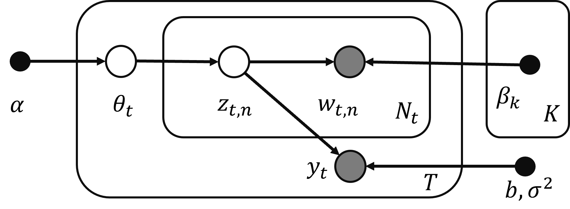
Figure 1: LDA Graphical Model
In specifying the response equation there are several modeling choices. Here we use a basic Gaussian response; however, (Blei and Mcauliffe (2008)) show how this response equation can be generalized to other members of the exponential family.
In the generative model we have assumed that the topic structure determines the response. It is possible to write a version of the response equation that uses \(\theta\) instead of \(\bar{Z}\). This would imply that documents and responses are exchangeable in the sense that once \(\theta\) is drawn we can first generate the document or the response. It makes more sense in the context of an application that seeks to extract information from news articles capable of changing market behavior and hence market outcomes to assume that documents are determined first followed by responses. Notice that so far (and in the details below) that the strategy would be the same if \(y\) is a response containing information for other economic variables, suggesting that we can think of supervised topic extraction with GDP, inflation, trade, unemployment, and other macroeconomic variables.
Variational Inference
The next natural step is to wonder how when given data we can use the previous framework to learn/estimate the parameters involved. The main challenge is the presence of two latent variables, namely \(\theta\) that controls document topic membership and the words’ topic assignments \(\{z_n\}\). The posterior distribution of the latent variables is given by:
\[\begin{equation} p(\theta,z_{1:N}|w_{1:N},y,\alpha,\beta_{1:K},b,\sigma^2)=\frac{p(\theta|\alpha)\left( \prod_{n=1}^N p(z_n|\theta)p(w_n|z_n \beta_{1:K})\right) p(y|z_{1:N},b,\sigma^2)}{\int \sum_{z_{1:N}} p(\theta|\alpha)\left( \prod_{n=1}^N p(z_n|\theta)p(w_n|z_n \beta_{1:K})\right) p(y|z_{1:N},b,\sigma^2) d\theta} \end{equation}\]
The normalizing term in the posterior distribution of the latent variables is the likelihood of the data \(p(w_{1:N},y|\pi)\). Unfortunately this likelihood is not efficiently computable, as documented in Blei et al (2003), making the posterior of the latent variables also not efficiently computable. If this posterior were computationally tractable we could use a standard EM algortihm to perform maximum likelihood and estimate the parameters.
Given this limitation, we resort to approximate maximum-likelihood estimation using a variational expectation maximization (VEM) strategy where we treat parameters \(\pi\) as constants to be estimated rather than random variables. The VEM strategy follows the spirit of the traditional EM algorithm but we use a variational approximation to the complete likelihood to find a maximizing set of parameters as our estimates. Notice the hybrid approach to parameters in this strategy: latent variables that can be thought of as observation-specific parameters have a Bayesian structure with priors on them, whereas common latent variables or global parameters are treated as unknown constants.
Evidence Lower Bound
To obtain an approximation of the complete likelihood in the presence of latent variables, we resort to the Evidence Lower Bound (ELBO), a key object in variational inference. Let \(q(\theta,z_{1:N})\) denote the for our latent variables (topic memberships and word assignments). By appropriately selecting the family of the variational distribution, we are able to approximate the likelihood. The log likelihood of the observed data is given by:
\[\begin{align*} \log p(w_{1:N},y|\pi)&=\log \int_\theta \sum_{z_{1:N}} p(w_{1:N},y,\theta,z_{1:N}|\pi)d\theta \\ &= \log\left( \int_\theta \sum_{z_{1:N}} p(w_{1:N},y,\theta,z_{1:N}|\pi) \frac{q(\theta,z_{1:N})}{q(\theta,z_{1:N})} d\theta\right)\\ &\geq E_q[\log p(w_{1:N},y,\theta,z_{1:N}|\pi)]-E_q[\log q(\theta,z_{1:N})] \end{align*}\]
Expectations in the last line are with respect to \(q(\theta,z_{1:N})\). This last line is the Evidence Lower Bound (ELBO). Denoting the entropy of the variational distribution as \(H(q)=-E_q[\log q(\theta,z_{1:N})]\) the ELBO for sLDA expands into: \[\begin{align*} \text{ELBO}&=E_q[\log p(w_{1:N},y,\theta,z_{1:N}|\pi)]+H(q)\\ &=E_q[\log p(\theta, z_{1:N}|w_{1:N},y,\pi)]+E_q[\log p(w_{1:N},y|\pi)]+H(q)\\ &=E_q[\log p(\theta|\alpha)]+\sum_{n=1}^N E_q[\log p(z_n|\theta)]+\sum_{n=1}^N E_q[\log p(w_n|z_n,\beta_{1:K})]\\ &+E_q[\log p(y|z_{1:N},b,\sigma^2)]+H(q)+E_q[\log p(w_{1:N},y|\pi)] \end{align*}\]
Notice that the ELBO is just a function of data \((w_{1:N},y)\) and the variational distribution \(q\). This bound is tight when \(q\) is the posterior of the latent variables, since maximizing the ELBO is equivalent to minimizing the Kullback-Leibler divergence between the posterior and \(q\), (see Blei et al (2017)). However, this posterior is computationally intractable so we approximate it.
Next, we take a stance on the family of the variational distribution and use mean-field variational inference to specify a fully factorized distribution: \[\begin{equation} q(\theta, z_{1:N}|\gamma,\phi_{1:N})=q(\theta|\gamma)\prod_{n=1}^{N}q(z_n|\phi_n) \end{equation}\]
In this fully factorized distribution \(\gamma\) is a \(K\)-dimensional Dirichlet parameter and each \(\phi_n\) parametrizes a K-dimensional multinomial distribution. Tightening the bound with respect to this factorized distribution is again equivalent to finding the member in this family that is closest in KL divergence to the posterior of the latent variables. Although the mean-field family for \(q\) is a common choice in variational inference, it is not the only family studied, see for example Wiegerinck and Barber (1999) who consider a family allowing for dependencies between the variables.
Within this family, our goal is to find \((\gamma, \phi_{1:N})\) that maximize the ELBO. Since the last term of the ELBO does not depend on the variational distribution our objective function is: \[\begin{align} \mathcal{L}(\gamma, \phi_{1:N})&=E_q[\log p(\theta|\alpha)]+\sum_{n=1}^N E_q[\log p(z_n|\theta)]+\sum_{n=1}^N E_q[\log p(w_n|z_n,\beta_{1:K})] \nonumber \\ &+E_q[\log p(y|z_{1:N},b,\sigma^2)]+H(q) \end{align}\]
Components of the ELBO \(\mathcal{L}(\gamma, \phi_{1:N})\)
Before optimizing \(\mathcal{L}\) we explicitly show each of its components:
\(E_q[\log p(\theta|\alpha)]\): Since \(\theta|\alpha\sim Dir(\alpha)\) we have that \(p(\theta|\alpha)=\left[\frac{\prod_{i=1}^K \Gamma(\alpha_i)}{\Gamma\left(\sum_{i=1}^K \alpha_i\right)}\right]\prod_{i=1}^K \theta_i^{\alpha_i-1}\) then:
\[\begin{align*} \log p(\theta|\alpha)&= \log \Gamma\left(\sum_{i=1}^K \alpha_i \right)-\sum_{i=1}^K \log \Gamma (\alpha_i)+\sum_{i=1}^K (\alpha_i-1)\log \theta_i\\ \text{and } E_q[\log p(\theta|\alpha)]&=\log \Gamma\left(\sum_{i=1}^K \alpha_i \right)-\sum_{i=1}^K \log \Gamma (\alpha_i)+\sum_{i=1}^K (\alpha_i-1)E_q[\log \theta_i]\\ \text{ where } E_q[\log \theta_i]&=\psi(\gamma_i)-\psi\left(\sum_{i=1}^K \gamma_i\right) \end{align*}\]
where \(\psi\) denotes the Digamma function.
\(E_q[\log p(z_n|\theta)]\): We assumed that \(z_n|\theta\sim Mult(\theta)\). Coding \(z_n\) in one-in-K form we can write \(p(z_n|\theta)=\prod_{i=1}^K \theta_i^{z_{n,i}}\), then \(\log p(z_n|\theta)=\sum_{i=1}^K z_{n,i}\log \theta_i\) and
\[\begin{align*} E_q[\log p(z_n|\theta)]=\sum_{i=1}^K E_q[z_{n,i}]E_q[\log \theta_i]=\sum_{i=1}^K \phi_{n,i} E_q[\log \theta_i] \end{align*}\]
\(E_q[\log p(w_n|z_n,\beta_{1:K})]\): Recall that \(w_n\in \{1,...,V\}\) and that \(\beta_{1:K}\) is \(V\times K\) matrix so we can write \(p(w_n|z_n,\beta_{1:K})=\prod_{i=1}^K \beta_{w_n,i}^{z_n,i}\) so we have:
\[\begin{align*} E_q[\log p(w_n|z_n,\beta_{1:K})]=\sum_{i=1}^K \phi_{n,i} \log \beta_{w_n,i} \end{align*}\]
\(E_q[\log p(y|z_{1:N},b,\sigma^2)]\): in the case of a gaussian response \(y=\bar{Z}'b+\varepsilon\) with \(\varepsilon\sim N(0,\sigma^2)\) we have:
\[\begin{align*} p(y|z_{1:N},b,\sigma^2)&=\frac{1}{\sqrt{2\pi \sigma^2}}\exp\left(-\frac{(y-\bar{Z}'b)^2}{2\sigma^2} \right)\\ \Rightarrow \log p(y|z_{1:N},b,\sigma^2)&= -\frac{1}{2}\log(2\pi \sigma^2)-\frac{1}{2\sigma^2} (y-\bar{Z}'b)^2\\ \text{ and } E_q[\log p(y|z_{1:N},b,\sigma^2)]&=-\frac{1}{2}\log(2\pi \sigma^2)-\frac{1}{2\sigma^2}\left[y^2-2yE_q[\bar{Z}]'b+b'E_q[\bar{Z}\bar{Z}']b\right] \end{align*}\]
To compute the previous expression we need \(E_q[\bar{Z}]\) and \(E_q[\bar{Z}\bar{Z}']\):
\[\begin{align*} E_q[\bar{Z}]&=\frac{1}{N}\sum_{n=1}^N \phi_n\\ E_q[\bar{Z}\bar{Z}']&=\frac{1}{N^2} \left(\sum_{n=1}^N \sum_{m\neq n} \phi_n\phi_m'+\sum_{n=1}^N diag(\phi_n)\right) \end{align*}\]
For the last we use that for \(n\neq m\), \(E_q[z_n z_m']=E_q[z_n]E_q[z_m']=\phi_n\phi_m'\) and that \(E[z_nz_n']=diag(E[z_n])=diag(\phi_n)\). Here \(diag(x)\) stands for put in a diagonal matrix the entries of the vector \(x\).
\(H(q)\): the entropy of the variational distribution is given by :
\[\begin{align*} H(q)&=-E_q[\log q(\theta,z_{1:N})]=-E_q[\log q(\theta|\gamma)]-\sum_{i=1}^n E_q[\log q(z_n|\phi_n)]\\ &=\log \Gamma\left(\sum_{i=1}^K \gamma_i \right)-\sum_{i=1}^K \log \Gamma (\gamma_i)+\sum_{i=1}^K (\gamma_i-1)E_q[\log \theta_i]-\sum_{n=1}^N\sum_{i=1}^K\phi_{n,i}\log \phi_{n,i} \end{align*}\]
Maximization of \(\mathcal{L}(\gamma, \phi_{1:N})\)
The optimization is done by block coordinate-ascent variational inference, that means iteratively maximizing \(\mathcal{L}\) with respect to each variational parameter. In this maximization we need to include the constraint that each of the multinomial parameters \(\phi_n\) should sum up to one.\
First we obtain the partial derivative of \(\mathcal{L}\) with respect to \(\gamma_i\) for \(i=1,...,K\)
\[\begin{align*} \frac{\partial \mathcal{L}}{\partial \gamma_i}&=\frac{\partial}{\partial \gamma_i}E_q[\log p(\theta|\alpha)]+\frac{\partial}{\partial \gamma_i} \sum_{n=1}^N E_q[\log p(z_n|\theta)]+\frac{\partial}{\partial \gamma_i}H(q)\\ &=(\alpha_i-1)\frac{\partial E[\log \theta_i]}{\partial \gamma_i}+\sum_{n=1}^N \phi_{n,i} \frac{\partial E[\log \theta_i]}{\partial \gamma_i}-\psi\left(\sum_{i=1}^K \gamma_i\right)+\psi(\gamma_i)-E_q[\log \theta_i]-(\gamma_i-1)\frac{\partial E[\log \theta_i]}{\partial \gamma_i}\\ &=\left[\alpha_i-\gamma_i+\sum_{n=1}^N \phi_{n,i} \right]\frac{\partial E[\log \theta_i]}{\partial \gamma_i}\\ \Rightarrow \frac{\partial \mathcal{L}}{\partial \gamma_i}&=0 \Leftrightarrow \gamma_i=\alpha_i+\sum_{n=1}^N \phi_{n,i} \end{align*}\] So we can update the whole vector: \[\begin{equation} \gamma^{new}\leftarrow \alpha+\sum_{n=1}^N \phi_n \end{equation}\]
Notice that this step is exactly the same as in the LDA VEM update. Next we obtain the partial derivative with respect to \([\phi_{n,i}]\) for \(i=1,...,K\) and \(n=1,...,N\)
\[\begin{align*} \frac{\partial \mathcal{L}}{\partial \phi_{n,i}} &= E_q[\log \theta_i]+\log \beta_{w_n,i}-\log \phi_{n,i}-1+\lambda+\frac{\partial}{\partial \phi_{n,i}}E_q[\log p(y|z_{1:N},b,\sigma^2)] \end{align*}\]
where \(\lambda\) is the Lagrange multiplier for the sum up to one constraint. The last partial derivative requires more work: \[\begin{align*} \frac{\partial}{\partial \phi_{n,i}}E_q[\log p(y|z_{1:N},b,\sigma^2)]=\frac{yb_i}{N\sigma^2}-\frac{1}{2\sigma^2}\frac{\partial}{\partial \phi_{n,i}} \left(b'E_q[\bar{Z}\bar{Z}']b\right) \end{align*}\] Let \(\phi_{-n}:=\sum_{m\neq n} \phi_m\); the trick here is to express \(b'E_q[\bar{Z}\bar{Z}']b\) as a function of just \(\phi_n\):
\[\begin{align*} f(\phi_n)&=\frac{1}{N^2} b'[\phi_n\phi_{-n}'+\phi_{-n}\phi_n'+diag(\phi_n)]b+\text{const.}\\ &= \frac{1}{N^2}[2(b'\phi_{-n})b'\phi_n+(b\cdot b)'\phi_n]+\text{const.}\\ \Rightarrow \frac{\partial}{\partial \phi_{n,i}} \left(b'E_q[\bar{Z}\bar{Z}']b\right) &= \frac{1}{N^2}[2(b'\phi_{-n})b+b\cdot b] \end{align*}\] Substituting this and noticing that \(\lambda\) acts as a normalization constant then:
\[\begin{align*} \frac{\partial \mathcal{L}}{\partial \phi_{n,i}}=0 \Leftrightarrow \phi_{n,i} \propto\exp\left[ E_q[\log \theta_i]+\log \beta_{w_n,i}+\frac{yb_i}{N\sigma^2}-\frac{1}{2\sigma^2 N^2}[2(b_i'\phi_{-n})b_i+b_i\cdot b_i] \right] \end{align*}\]
and updating the whole vector is done by:
\[\begin{equation} \phi_n^{new}\propto \exp\left[E_q[\log \theta]+\log \beta_{w_n,\cdot}+\frac{yb}{N\sigma^2}-\frac{1}{2\sigma^2 N^2}[2(b'\phi_{-n})b+b\cdot b] \right] \end{equation}\] here the proportional stands for compute each entry and then normalize to one.\
Using these updates iteratively we can find local maximizers \(\{\gamma, \phi_{1:N}\}\) of the ELBO for a given document-response pair and a set of parameters \(\pi=\{\alpha,\beta_{1:K},b,\sigma^2\}\).
Maximization of \(L(\pi)\)
Once we have maximizers \(\{\gamma, \phi_{1:N}\}\) of the ELBO for each given document-response pair, we are ready to update the global parameters \(\pi=\{\alpha,\beta_{1:K},b,\sigma^2\}\) in the M-step by maximizing \(L(\pi)\), the corpus-level ELBO. In this step we want to maximize over \(\pi\) the objective function:
\[\begin{align*} L(\pi)&=\sum_{t=1}^T E_{q_t}[\log p(\theta_t,z_{t,1:N_t}, w_{t,1:N_t},y_t)|\pi]+H(q_t)\\ &=\sum_{t=1}^T \mathcal{L}(\gamma_t, \phi_{t,1:N_t}; w_{t,1:N_t},y_t,\pi) \end{align*}\]
Here each term in the sum is the \((w_{t,1:N_t},y_t)\) specific ELBO evaluated at the corresponding maximizing \(\{\gamma_t^*, \phi_{t,1:N_t}^*\}\) from the E-step. The optimizing value for topic \(k\) and work \(w\) in the topic matrix, \(\beta_{w,k}\) is given by:
\[\begin{align} \frac{\partial L}{\partial \beta_{w,k}}&=\sum_{t=1}^T \sum_{n=1}^{N_t} \mathbb{I}\{w_{t,n}=w\}\phi_{t,n,k}\frac{1}{\beta_{w,k}}-\lambda=0 \nonumber\\ \Rightarrow \beta_{w,k} &\propto \sum_{t=1}^T \sum_{n=1}^{N_t} \mathbb{I}\{w_{t,n}=w\}\phi_{t,n,k} \end{align}\]
The topic membership hyper parameter \(\alpha\) is treated as hyper parameter chosen by the econometrician. For example it is common to set it at \(\alpha=1/K\). For the response coefficient \(b\):
\[\begin{align} \frac{\partial L}{\partial b}&=\sum_{t=1}^T \frac{\partial }{\partial b} E_q[\log p(y_t|z_{t,1:N_t},b,\sigma^2)] =\sum_{t=1}^T \frac{1}{\sigma^2}\left[ y_t E_q[\bar{Z}_t]'-b'E_q[\bar{Z}_t\bar{Z}_t'] \right]=0 \nonumber\\ \Rightarrow b&= \left(\sum_{t=1}^T E_q[\bar{Z}_t\bar{Z}_t']\right)^{-1}\left( \sum_{t=1}^T E_q[\bar{Z}_t]'y_t\right) \end{align}\]
Detailed expressions for \(E_q[\bar{Z}_t\bar{Z}_t']\) and \(E_q[\bar{Z}_t]'y_t]\) are the ones shown in the previous section. Finally the response dispersion coefficient \(\sigma^2\) is optimizer is given by:
\[\begin{align} \frac{\partial L}{\partial b}&=\sum_{t=1}^T \frac{\partial }{\partial \sigma^2} E_q[\log p(y_t|z_{t,1:N_t},b,\sigma^2)] =\sum_{t=1}^T -\frac{1}{2\sigma^2}+\frac{1}{2\sigma^4} E_q[(y_t-\bar{Z}_t'b^{new})^2]=0 \nonumber\\ \Rightarrow \sigma^2&= \frac{1}{T}\sum_{t=1}^T \left( y_t^2-y_tE_q[\bar{Z}_t']b^{new}\right) \end{align}\]
Parameter Estimation
We now look for parameters \(\pi=\{\alpha, \beta_{1:K},b,\sigma^2\}\) that maximize the corpus-level ELBO in (); this is done via the VEM algorithm, that iteratively performs the E-Step and M-Step described below.
E-Step
In the E-step given a set of parameters from the previous iteration, we approximate the likelihood of the data by maximizing each document-specific ELBO, and then summing them into \(L(\pi)\) as described in the previous section. In this step the goal is to find a collection \(\{\gamma_t, \phi_{t,1:N}\}\) that maximizes each document-specific ELBO using CAVI. Optimization boils down to iteratively updating \(\{\gamma, \phi_{1:N}\}\) for each document as: \[\begin{align} \label{updateGamma} \gamma^{new}&\leftarrow \alpha+\sum_{n=1}^N \phi_n \\ \label{updatePhi} \phi_n^{new} &\propto \exp\left[E_q[\log \theta]+\log \beta_{w_n,\cdot}+\frac{yb}{N\sigma^2}-\frac{1}{2\sigma^2 N^2}[2(b'\phi_{-n})b+b\cdot b] \right] \end{align}\]
M-Step
In the the M-step we maximize the corpus ELBO with respect to the sLDA parameters \(\pi=\{\alpha, \beta_{1:K},b,\sigma^2\}\). The updates in this step boil down to:
\[\begin{align} \label{updateBeta} \beta_{w,k} &\propto \sum_{t=1}^T \sum_{n=1}^{N_t} \mathbb{I}\{w_{t,n}=w\}\phi_{t,n,k} \\ \label{updateB} b^{new}& \leftarrow \left(\sum_{t=1}^T E_q[\bar{Z}_t\bar{Z}_t']\right)^{-1}\left( \sum_{t=1}^T E_q[\bar{Z}_t]'y_t\right)\\ \label{updateSigma} \sigma^2& \leftarrow \frac{1}{T}\sum_{t=1}^T \left( y_t^2-y_tE_q[\bar{Z}_t']b^{new}\right) \end{align}\]
As mentioned above the VEM algorithm iteratively alternates these steps until convergence in the corpus-level ELBO in \(L(\pi)\) is achieved.
Response Prediction
In sLDA given a set of parameters \(\pi\) and a document, we can predict the response variable \(y\) associated with the document. Using a quadratic loss function, the prediction simplifies to computing the conditional expected value:
\[\begin{align*} E[y|w_{1:N},\pi]&=E[E[y|z_{1:N},b,\sigma^2]|w_{1:N},\alpha,\beta_{1:K}]=E[b'\bar{Z}|w_{1:N},\alpha,\beta_{1:K},b]\\ &=b'E[\bar{Z}|w_{1:N},\alpha,\beta_{1:K}] \end{align*}\]
To compute the last conditional expectation we resort again to variational inference and compute the posterior mean of \(\bar{Z}\). The goal is to find a variational distribution \(\tilde{q}(\theta, z_{1:N})\) over the latent variables that minimizes the KL divergence between this distribution and the posterior distribution \(p(z_{1:N}|w_{1:N},\alpha,\beta_{1:K})\); this is equivalent again to maximizing the corresponding ELBO. This is similar to the ELBO maximization in sLDA but the difference is that terms involving the response variable \(y\) will not appear since this variable is averaged out. The variational updates are the same as in an unsupervised LDA model for \((\theta, z_{1:N})\).
Similarly, using a fully factorized variational distribution:
\[\begin{equation*} \tilde{q}(\theta, z_{1:N}|\tilde{\gamma},\tilde{\phi}_{1:N})=\tilde{q}(\theta|\tilde{\gamma})\prod_{n=1}^{N}\tilde{q}(z_n|\tilde{\phi}_n) \end{equation*}\]
the updates for maximizing the ELBO are:
\[\begin{align*} \tilde{\gamma}^{new}&\leftarrow \alpha+\sum_{n=1}^N \tilde{\phi}_n\\ \tilde{\phi}_n^{new}&\propto \exp\left[E_{\tilde{q}}[\log \theta]+\log \beta_{w_n,\cdot}\right] \end{align*}\]
where \(E_{\tilde{q}}[\log \theta_i]=\psi(\tilde{\gamma}_i)-\psi\left(\sum_{i=1}^K \gamma_i\right)\). Once the variational parameters have been optimized then:
\[\begin{align} E[\bar{Z}|w_{1:N},\alpha,\beta_{1:K}]&\approx E_{\tilde{q}}[\bar{Z}]=N^{-1}\sum_{n=1}^N \tilde{\phi}_i \nonumber\\ \Rightarrow E[y|w_{1:N},\pi]&\approx b'\left(N^{-1}\sum_{n=1}^N \tilde{\phi}_n\right) \end{align}\]
That is, we set \(\hat{y}=b'\left(N^{-1}\sum_{n=1}^N \tilde{\phi}_n\right)\) as our predicted response given a set of parameters \(\pi\) (or their corresponding estimates) and a document \(w_{1:N}\).