Building a DNN from scratch in Julia

This post shows how to build a deep neural network from scratch in Julia for the classic appication of building a clasifier of images of cats

Preamble

Some notes before start.

• This post is an adaptation from the application presented in Python language in the Andrew Ng’s Deep Learning, here I just parsed the Python code to Julia for my own learning.
• This is a more didactic approach to building a Deep Neural Network in Julia, where most pieces of the algorithm are coded from basic functions; however for serious deep learning the best option is using dedicated environments for machine learning like Flux. An introduction to Flux can be found here.
• The application presented is of computer vision, using an architecture from the computer vision literature will yield a NN with better accuracy, however, we use the basic pieces of a NN for didactic purposes.
• The data sets used can be downloaded here
• Executing Julia from RStudio: This blogpost is in R Markdown the Julia execution to knit this post is done using JuliaCall with the chunk’s language set up to julia, however the following functions can be executed directly on a Julia IDE, actually the first time I coded this exercise was in Atom customize to Juno.

The data

Julia set up in R

library(JuliaCall);
options(JULIA_HOME="C:/Users/aaron/AppData/Local/Programs/Julia-1.6.1/bin")
julia_setup(rebuild=TRUE)

#Test code in Julia
a=sqrt(2);
println(a)

1.4142135623730951

Load the Data

This functions uses load_data() an auxiliary function presented in the appendix of auxiliary functions, here.

using HDF5, Images, ImageView, TestImages
#---------- Load the data
trset_x_orig, trset_y_orig, tset_x_orig, tset_y_orig, classes=load_data()
#Example Image: The index can be changed by the user
ExampleIm=trset_x_orig[:,:,:,129];
#Convert the UInt8 hexadecimal format to N0f8 (ranging from 0 to 1)
B=normedview(ExampleIm);
C=colorview(RGB,B[1,:,:],B[2,:,:],B[3,:,:])'
imshow(C);

Image with index 129 is the following image of a cat, in Julia is represented as an 3x64x64 array, a image of 64-by-64 pixels in 3 channels, RGB.

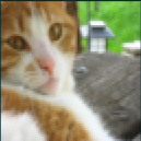
Figure 1: An example image from the training set

Preprocess the Data

In this step, we create a function to flatten the data into a vector (from a 3-dimensional array) and normalize by 255 to have pixel values between zero and one.

#Function to vectorize the images
function flatData(X::Array)
    flatX=reshape(X, :, size(X)[end])/255
    return flatX
end

trset_x=flatData(trset_x_orig);
tset_x=flatData(tset_x_orig);

Here we have 209 images in the training set and 50 images in the test set.

The ingredients/design

Number of layers and neurons per layer

We are going to use a 5-layer NN (four hidden layers) with:

• First hidden layer with 20 neurons
• Second hidden layer with 15 neurons
• Third hidden layer with 10 neurons
• Fourth hidden layer with 5 neurons
• Fifth/final layer with 1 neuron

We specified this architecture into an array with the dimensions of the weights matrices per layer. We also use init_param(), presented here to initialize the parameters of the NN.

dim_layers=[size(trset_x)[1],20,15,10,5,1];
Param=init_param(dim_layers);

For example, this implies that in the first layer, the weight matrix \(W_1\) is \(20\times 12288\) because we take the flatten image of the input layer (\(3\cdot 64\cdot 64=12288\)) and we multiply by the weights in each of the 20 neurons; the associated bias is \(b_1\) that is \(20\times 1\). In the second layer, the weight matrix \(W_2\) is \(15\times 20\) because we take the output from the first layer (\(20\times 1\)) and we multiply by the weights in each of the 15 neurons of the second layer; the associated bias is \(b_2\) that is \(15\times 1\).

In this model our parameters to learn are \((W_i,b_i)\) with \(i=1,2,3,4,5\). That amount to \(258,316\) constants to optimize (\(12888\cdot 20+20+15\cdot 20+15+10\cdot 15+10+5\cdot 10+5+5\cdot 1+1\)).

Loss Function

We are going to use the cross entropy cost functions. It is implemented here. Let \(\hat{a}\) be the output vector from the last layer of the NN; then the cost functions is given by: \[C=-\frac{1}{N}\sum_{i=1}^N y_i \ln(\hat{a}_i)+(1-y_i)\ln(1-\hat{a}_i)\] where \(N\) is the number of examples in the training set.

Activation Functions

We will use two activation functions: in the first 4 hidden layers each neuron will use a ReLu activation and in the final layer the activation will be of the Sigmoid function.

The ReLU function is implemented here and it is given by: \[f(x)=\max(0,x)\]

The Sigmoid function is implemented here and it is given by: \[\sigma(x)=\frac{1}{1+\exp(-x)}\] Notice that the sigmoid function is always between zero and one.

Number of Iterations

During training we will do \(S=10000\) iterations, where each iterations performs a forward propagation, computes the associated cost, does backward propagation and finally updates the parameters before the following iteration. Performing a fixed number of iterations during optimization is rather simple, it would be better to create a flag that stops execution after achieving a target accuracy in the training sample.

Learning Rate

When optimizing using gradient descent, a learning rate \(\alpha\) is used during the parameter update:

\[\theta_{t+1}\leftarrow\theta_t+\alpha \frac{\partial C}{\partial \theta}\bigg\rvert_{\theta=\theta_t}\]

In this exercise we set \(\alpha=0.0075\). There is whole literature about the role of the learning rate and how to set it.

Model Training

Training the model will be done using gradient descent to optimize the cost function. This entails:

1. Set initial values for the parameters::. \(W_i^0, b_i^0\) for \(i=1,2,3,4,5\). Implementation here
2. In each of the iterations:

• Do a forward propagation with current parameters. Implementation here.
• Compute the value of the loss function with current parameters. Implementation here.
• Do a backward propagation. Implementation here.
• Update parameters before next iteration. Implementation here.
• Report latest cost for monitoring execution.

3. Return optimized parameters.

These steps are combined in the following L_layer_model() function.

"""
Function to combine all sustantive function into a deep cat classifier
"""
function L_layer_model(X::Array,Y::Array,layer_dims::Array, learning_rate::Float64,num_iter::Int,print_cost::Bool)
    #Step 1: Initialize parameters
    param=init_param(layer_dims); println(param["W1"][1:2,1:2])
    #Step 2: Gradient descent loop
    for i in 1:num_iter
        #Step 3: Do a complete forward pass
        AL,caches=complete_forward(X, param)
        #Step 4: Compute the current cost
        cost=cost_function(AL,Y)
        #Step 5: Do a complete backward pass
        grads=complete_backward(AL,Y,caches)
        #Step 6: Update parameters
        param=update_param(param,grads,learning_rate)
        #Step 7: Print cost
        if print_cost & ((i%100)==0)
            println("The cost after iteration ", i , " is ",cost)
            println(param["W1"][1:2,1:2])
        end
    end
    #Step 8: Return the parameters
    return param
end

lrate=0.0075; nIter=10000;
#Train the model
@time parameters=L_layer_model(trset_x,trset_y,
                                dim_layers, lrate, nIter, true)

Executing the function with 10000 iterations should not take long (under a couple of minutes) and in the execution we should see the cost function values decreasing.

Assessing Accuracy

The next step is to evaluate the accuracy of the model in both the training and the test set. We use the predict() function implemente here. In this functions if the predicted probability of \(Y=1\), is bigger than 50%, then we label that image as of a cat, and if the probability is less than 50% then it is labelled as of not a cat. This threshold can be adjusted according the application, here we opt for a parsimonious approach.

#Check the Accuracy on the train set
pred_train = predict(trset_x, trset_y, parameters)

#Check the Accuracy on the test set
tset_y=reshape(tset_y_orig,(1,length(tset_y_orig)));
pred_test = predict(tset_x, tset_y, parameters)

The previous code gives an accuracy on the training set of \(99.52\%\) and of \(66\%\) on the test set, not bad for a NN without using computer vision tricks.

Training Accuracy: 0.9952153110047847
Test Accuracy: 66

Predicting an image

Finally we illustrate how the NN predicts an image in the test set.

index=50
Example_Test_Im=tset_x_orig[:,:,:,index];
#Convert the UInt8 hexadecimal format to N0f8 (ranging from 0 to 1)
B=normedview(Example_Test_Im);
C=colorview(RGB,B[1,:,:],B[2,:,:],B[3,:,:])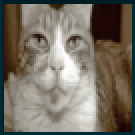

Figure 2: An example image from the test set

We see that the image is that of a cat, the NN has not seen this image and correctly identifies that the image has a cat!

if pred_test[index]==tset_y[index]
    println("Correct! The label is correct.")
    if pred_test[index]==1
        println("It's a CATTO! "); println("It's a CATTO! "); println("It's a CATTO! ")
    elseif pred_test[index]==0
        println("No Cat! "); println("No Cat! "); println("No Cat! ")
    end
else
    println("!!! The label is incorrect !!!")
end

Correct! The label is correct.
It's a CATTO!
It's a CATTO!
It's a CATTO!

Auxiliary Functions

Load data

The h5 files are in a folder named datasets.

#Function to read the h5 file and obtain the matrices for the images
function load_data()
    #Train data
    train_data=h5open("datasets\\train_catvnoncat.h5","r")
    train_set_x_orig=read(train_data["train_set_x"]) # your train set features
    train_set_y_orig=read(train_data["train_set_y"]) # your train set labels
    #Test data
    test_data=h5open("datasets\\test_catvnoncat.h5","r")
    test_set_x_orig=read(test_data["test_set_x"]) # your train set features
    test_set_y_orig=read(test_data["test_set_y"]) # your train set labels
    #Classes
    classes=read(test_data["list_classes"])
    #Reshape the matrices
    return train_set_x_orig, train_set_y_orig, test_set_x_orig, test_set_y_orig, classes
end

Sigmoid Functions

#Computes the Sigmoid function to the entries of the array A

function Sigmoid(A::Array)
    cache=A
    Z=(exp.(-A).+1).^(-1)
    return Z,cache
end

#sigmoid backward

function sigmoid_backward(dA::Array,cache::Array)
  Z=reshape(cache,size(dA));
  S=(exp.(-Z).+1).^(-1);
  dZ=dA.*(S.*(-S.+1));
  @assert size(dZ)==size(Z)
  return dZ
end

ReLu Functions

#ReLu Function
#Computes the ReLU activation function to the entries of the array A

function ReLu(A::Array)
    cache=A
    Z=max.(A,0)
    @assert size(A)==size(Z)
    return Z,cache
end

#Relu backward
function relu_backward(dA::Array,cache::Array)
Z=cache; dZ=copy(dA); dZ[Z.<0].=0;
@assert size(dZ)==size(Z)
return dZ
end

Substantive functions

Initialize Parameters

#Parameter initializing
"""
Function to initialize the parameter of all the layers
"""
function init_param(layer_dim::Array)
    param=Dict();
    for l in 2:length(layer_dim)
        param[string("W",(l-1))]=randn((layer_dim[l],layer_dim[l-1]))/sqrt(layer_dim[l-1]);
        param[string("b",(l-1))]=zeros(layer_dim[l],1)
        @assert size(param[string("W",(l-1))])==(layer_dim[l], layer_dim[l-1])
        @assert size(param[string("b",(l-1))])==(layer_dim[l],1)
    end
    return param
end

Linear activation

#Forward Linear Activation
"""
Function to compute the forward linear activation of a layer
"""
function linear_activation(A_prev::Array, W::Array, b::Array, activation::String)
linear_cache=Dict("A_prev"=>A_prev,"W"=>W,"b"=>b);
Z=W*A_prev.+b;
if activation=="sigmoid"
    A,act_cache=Sigmoid(Z)
elseif activation=="relu"
    A,act_cache=ReLu(Z)
end
cache=Dict("LinCache"=>linear_cache,"ActCache"=>act_cache)
return A,cache
end

Complete forward

#Complete forward propagation
function complete_forward(X::Array, parameters::Dict)
    A=X
    L=Int(length(parameters)/2)
    caches=[]
    for l in 1:(L-1)
        A_prev=A
        A,cache=linear_activation(A_prev,parameters[string("W",l)], parameters[string("b",l)], "relu")
        caches=vcat(caches,cache)
    end
    AL,cache=linear_activation(A,parameters[string("W",L)], parameters[string("b",L)], "sigmoid")
    caches=vcat(caches,cache)
    return AL, caches
end

Cost Function

"""
Function for the cross entropy cost
"""
function cost_function(AL::Array,Y::Array)
  m=length(Y)
  cost=(-1/m)*sum(Y.*log.(AL).+(-Y.+1).*log.(-AL.+1))
  return cost
end

Linear backward

#Linear_backward step
"""
Function to compute one step of linear-backward derivatives
"""
function Linear_backward(dZ::Array,cache::Dict)
  A_prev=cache["A_prev"]; W=cache["W"]; b=cache["b"];
  m=size(A_prev)[2]; #dZ=reshape(dZ,(1,length(dZ)))
  dW=(1/m)*dZ*A_prev'
  db=(1/m)*sum(dZ,dims=2)
  dA_prev=W'*dZ
  
  @assert size(A_prev)==size(dA_prev)
  @assert size(W)==size(dW)
  @assert size(b)==size(db)
  
  return dA_prev,dW,db
end

Linear activation backward

#Linear activation backward
"""
Function to compute the backward prop of a linear activation layer
"""
function linear_act_back(dA::Array,cache::Dict,activation::String)
  linear_cache=cache["LinCache"]
  activation_cache=cache["ActCache"]
  if activation=="relu"
      dZ=relu_backward(dA, activation_cache);# print(dZ)
      dA_prev, dW, db=Linear_backward(dZ, linear_cache)
  elseif activation=="sigmoid"
      dZ=sigmoid_backward(dA, activation_cache);# print(dZ)
      dA_prev, dW, db=Linear_backward(dZ, linear_cache)
  end
  return dA_prev, dW, db
end

Complete Backward

"""
Function that computes the whole backward pass
"""
function complete_backward(AL::Array,Y::Array,caches::Array)
  grads=Dict()
  L=length(caches)
  #AL=reshape(AL,m);
  Y=reshape(Y,(1,length(Y)))
  #Initialize the back prop
  dAL=-((Y./AL)-(-Y.+1)./(-AL.+1))
  current_cache=caches[L]
  grads[string("dA",L)], grads[string("dW",L)], grads[string("db",L)] = linear_act_back(dAL, current_cache, "sigmoid")
  #Do the whole backward pass
  for l in 1:(L-1)
  current_cache=caches[(L-l)]
  dA_prev_temp, dW_temp, db_temp = linear_act_back(grads[string("dA",(L-l+1))], current_cache, "relu")
  grads[string("dA",(L-l))]=dA_prev_temp
  grads[string("dW",(L-l))]=dW_temp
  grads[string("db",(L-l))]=db_temp
  end
  return grads
end

Update parameters

#Function to update parameters
"""
Function to update the parameters via gradient descent
"""
function update_param(param::Dict, grads::Dict, learning_rate::Float64)
  L=Int(length(param)/2)
  for l in 1:L
      param[string("W",l)]=param[string("W",l)]-learning_rate*grads[string("dW",l)]
      param[string("b",l)]=param[string("b",l)]-learning_rate*grads[string("db",l)]
  end
  return param
end

Construct Predictions

#Function to construct predictions given parameters
function predict(X::Array,Y::Array,param::Dict)
  m=size(X)[2]
  probs,caches=complete_forward(X,param)
  p=1*(probs.>0.5)
  acu=sum(p.==Y)/m
  println("Probs: ", string(probs))
  println("Predictions: ", string(p))
  println("True labels: ", string(Y))
  println("Accuracy: ",acu)
  return p
end